Autocatalytic Networks

Autocatalytic Networks with `lifesimulatoR`

This tutorial introduces autocatalytic networks. In origin-of-life research, autocatalysis is important because it offers a possible route from ordinary chemistry to self-sustaining chemical organization.

A catalyst is something that helps a reaction occur more easily without being consumed by the reaction. An autocatalytic system is one in which the products of reactions help produce more of themselves, either directly or indirectly. In a network, molecule A might help produce molecule B, molecule B might help produce molecule C, and molecule C might help produce molecule A. Together, the system can become self-reinforcing.

This idea matters because early life may not have begun with a single perfect self-replicator. It may have involved networks of mutually reinforcing chemical reactions. Life is not only about individual molecules; life also depends on systems of interaction. Modern cells contain large networks of reactions, enzymes, metabolites, and feedback loops. Autocatalytic network models provide a simplified way to explore how self-maintaining organization could emerge before modern biology.

library(lifesimulatoR)

What is an autocatalytic network?

An autocatalytic network is a system in which molecules help produce other molecules in the same system. Instead of one molecule simply copying itself, a group of molecules collectively supports its own production.

This shifts attention from individual molecules to systems of interactions. In such systems, persistence may emerge from the network as a whole.

This is different from a simple replication-first model, where the main focus is on a molecule that can copy itself.

Simulating a toy autocatalytic network

lifesimulatoR includes a simplified autocatalytic network model. The main function is autocatalytic_network().

network <- autocatalytic_network(
  n_types = 8,
  steps = 50,
  catalysis_probability = 0.2,
  seed = 123
)

names(network)

## [1] "time_series"      "catalysis_matrix"

The function creates a toy system with a number of molecular types and probabilistic catalytic relationships between them.

The returned object includes two main components:

time_series: a tibble showing molecular abundances over time.
catalysis_matrix: a matrix showing which molecular types catalyze others.

head(network$time_series)

## # A tibble: 6 × 3
##    step molecule abundance
##   <int> <chr>        <dbl>
## 1     0 M1           0.833
## 2     0 M2           0.504
## 3     0 M3           0.829
## 4     0 M4           0.831
## 5     0 M5           0.815
## 6     0 M6           0.496

network$catalysis_matrix

##       [,1]  [,2]  [,3]  [,4]  [,5]  [,6]  [,7]  [,8]
## [1,] FALSE FALSE FALSE FALSE FALSE  TRUE FALSE  TRUE
## [2,] FALSE FALSE  TRUE FALSE FALSE FALSE FALSE FALSE
## [3,] FALSE FALSE FALSE FALSE  TRUE FALSE  TRUE FALSE
## [4,] FALSE FALSE FALSE FALSE FALSE FALSE FALSE FALSE
## [5,] FALSE FALSE FALSE FALSE FALSE  TRUE FALSE FALSE
## [6,]  TRUE FALSE FALSE  TRUE FALSE FALSE  TRUE  TRUE
## [7,] FALSE  TRUE FALSE FALSE FALSE FALSE FALSE FALSE
## [8,] FALSE FALSE FALSE FALSE FALSE FALSE FALSE FALSE

Understanding the parameters

The main arguments are:

n_types: the number of molecular types in the system.
steps: the number of simulation steps.
catalysis_probability: the probability that one molecule type catalyzes another.
seed: an optional random seed for reproducibility.

The catalysis_probability parameter is especially important. If this value is very low, few catalytic connections form. If it is higher, the network becomes more connected.

In origin-of-life theory, the emergence of a sufficiently connected catalytic network may be a key transition.

Why network connectivity matters

A set of isolated molecules may react occasionally, but it may not sustain itself. A connected network can create feedback. Once feedback exists, some molecular systems may persist longer, grow faster, or resist disappearance.

The simplified question is:

At what point does a random chemical network become organized enough to support self-sustaining dynamics?

This is not only a chemistry question. It is also a systems question. The structure of the network matters.

Time series output

The time_series output can be used to track how the system changes over time.

head(network$time_series)

## # A tibble: 6 × 3
##    step molecule abundance
##   <int> <chr>        <dbl>
## 1     0 M1           0.833
## 2     0 M2           0.504
## 3     0 M3           0.829
## 4     0 M4           0.831
## 5     0 M5           0.815
## 6     0 M6           0.496

summary(network$time_series)

##       step      molecule           abundance       
##  Min.   : 0   Length:408         Min.   :  0.4959  
##  1st Qu.:12   Class :character   1st Qu.:  3.8842  
##  Median :25   Mode  :character   Median : 16.7127  
##  Mean   :25                      Mean   : 48.5247  
##  3rd Qu.:38                      3rd Qu.: 65.6887  
##  Max.   :50                      Max.   :366.1732

Depending on the simulation settings, the time series may show whether some molecule types become more abundant than others.

Plotting one molecule type

We can use plot_simulation() to visualize the abundance of one molecule type through time.

m1 <- subset(network$time_series, molecule == "M1")

plot_simulation(m1, x = "step", y = "abundance")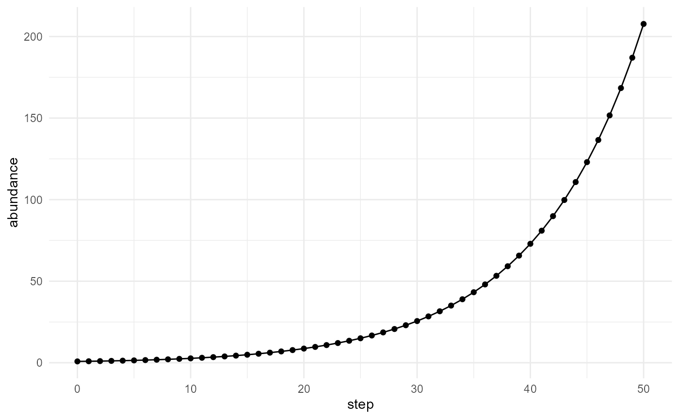

This plot shows how the abundance of molecule M1 changes through the simulation.

Summarizing final abundances

It is often useful to look at the final simulation step.

final_step <- max(network$time_series$step)

final_abundances <- subset(network$time_series, step == final_step)

final_abundances

## # A tibble: 8 × 3
##    step molecule abundance
##   <int> <chr>        <dbl>
## 1    50 M1            208.
## 2    50 M2            266.
## 3    50 M3            199.
## 4    50 M4            208.
## 5    50 M5            148.
## 6    50 M6            271.
## 7    50 M7            354.
## 8    50 M8            366.

This output shows which molecule types are most abundant at the end of the simulation.

Experiment 1: Low versus high catalysis probability

We can compare two networks: one with sparse catalytic connections and one with more frequent catalytic connections.

sparse_network <- autocatalytic_network(
  n_types = 8,
  steps = 50,
  catalysis_probability = 0.05,
  seed = 123
)

dense_network <- autocatalytic_network(
  n_types = 8,
  steps = 50,
  catalysis_probability = 0.4,
  seed = 123
)

head(sparse_network$time_series)

## # A tibble: 6 × 3
##    step molecule abundance
##   <int> <chr>        <dbl>
## 1     0 M1           0.833
## 2     0 M2           0.504
## 3     0 M3           0.829
## 4     0 M4           0.831
## 5     0 M5           0.815
## 6     0 M6           0.496

head(dense_network$time_series)

## # A tibble: 6 × 3
##    step molecule abundance
##   <int> <chr>        <dbl>
## 1     0 M1           0.833
## 2     0 M2           0.504
## 3     0 M3           0.829
## 4     0 M4           0.831
## 5     0 M5           0.815
## 6     0 M6           0.496

In a sparse network, many molecular types may have few or no catalytic relationships. In a denser network, feedback loops are more likely. This can make the system more dynamic and potentially more self-reinforcing.

Experiment 2: Compare final abundance patterns

sparse_final <- subset(
  sparse_network$time_series,
  step == max(sparse_network$time_series$step)
)

dense_final <- subset(
  dense_network$time_series,
  step == max(dense_network$time_series$step)
)

sparse_final

## # A tibble: 8 × 3
##    step molecule abundance
##   <int> <chr>        <dbl>
## 1    50 M1            6.12
## 2    50 M2            1.77
## 3    50 M3            6.13
## 4    50 M4            1.89
## 5    50 M5           14.0 
## 6    50 M6            1.77
## 7    50 M7           14.0 
## 8    50 M8            1.83

dense_final

## # A tibble: 8 × 3
##    step molecule abundance
##   <int> <chr>        <dbl>
## 1    50 M1          76522.
## 2    50 M2          66124.
## 3    50 M3          48509.
## 4    50 M4         156282.
## 5    50 M5         234561.
## 6    50 M6         225042.
## 7    50 M7         194458.
## 8    50 M8         221803.

This comparison helps illustrate how changing network connectivity may affect final molecular abundance.

Experiment 3: Increasing the number of molecular types

A larger system may allow more possible catalytic relationships.

larger_network <- autocatalytic_network(
  n_types = 15,
  steps = 50,
  catalysis_probability = 0.2,
  seed = 123
)

head(larger_network$time_series)

## # A tibble: 6 × 3
##    step molecule abundance
##   <int> <chr>        <dbl>
## 1     0 M1           0.456
## 2     0 M2           0.530
## 3     0 M3           0.604
## 4     0 M4           0.728
## 5     0 M5           0.924
## 6     0 M6           0.657

As n_types increases, the number of possible relationships grows. This can make the network more complex, even if the probability of each individual catalytic relationship stays the same.

Teaching interpretation

This model can be used to introduce the following ideas:

Mutual reinforcement
Chemical networks
Feedback loops
Collective self-maintenance
Emergence of system-level behaviour
Network connectivity
System-level selection

The key teaching point is that an origin-of-life model does not always need to begin with a single molecule that copies itself perfectly. It can also begin with interacting systems that collectively sustain themselves.

Autocatalysis and the origin of life

Autocatalytic networks are relevant to several origin-of-life hypotheses. Some theories suggest that life began not with a single self-replicating molecule, but with a network of mutually supporting reactions. This is often associated with metabolism-first or network-first perspectives.

In this view, the earliest life-like systems may have been chemical networks that could maintain themselves, process energy, and generate more components of the same network. Genetic replication may have become dominant later.

This contrasts with RNA World models, where the focus is often on molecules capable of both storing information and catalyzing reactions.

These views are not necessarily mutually exclusive. A mature origin-of-life theory may need to explain how networks, compartments, energy flows, and information-carrying molecules became coupled.

What this model includes and excludes

This simplified model includes:

Molecular types
Probabilistic catalytic relationships
Time evolution
Network-level behaviour
Abundance changes

It does not include:

Real reaction kinetics
Thermodynamic constraints
Spatial structure
Energy gradients
Detailed molecular chemistry
Realistic reaction pathways

For teaching purposes, this limitation is useful. It allows students to focus on the network concept before adding chemical detail.

Interpretation

The key idea is that autocatalytic networks shift the focus from individual molecules to systems of interaction. A molecule may not be impressive by itself, but a network of molecules can produce feedback, persistence, and organization.

This is one reason autocatalysis is such an important idea in origin-of-life research. It provides a possible bridge between random chemistry and the organized, self-maintaining systems seen in living organisms.

Suggested exercises

Run the model with different values of catalysis_probability.
Increase n_types and observe whether larger systems behave differently.
Compare short simulations and long simulations.
Plot several molecule types and compare their abundance trajectories.
Discuss how autocatalytic networks differ from simple molecular replication.
Propose one additional feature that would make the model more chemically realistic.
Discuss how autocatalytic networks might interact with protocells.
Compare network-first and replication-first views of the origin of life.

Interpretation caution

This is a conceptual network model, not a detailed chemical kinetics model. It is useful for exploring how feedback and catalytic relationships can produce system-level behaviour, but it should not be interpreted as a chemically realistic simulation of abiogenesis.