Diversity, Entropy, and Complexity
Source:vignettes/4. diversity-metrics.Rmd
4. diversity-metrics.RmdDiversity and Complexity Metrics with
lifesimulatoR
Why diversity matters
Diversity is important in origin-of-life simulations because a system with more molecular variety can explore more possibilities. A diverse molecular population may contain more potential structures, interactions, catalytic patterns, or replication-like behaviours.
However, diversity alone is not the same as life. A random chemical mixture can be highly diverse but poorly organized. A highly selected system may have lower diversity but stronger functional structure. For this reason, diversity metrics should be interpreted carefully. They are useful indicators, not complete measures of life or complexity.
In simplified origin-of-life models:
- Mutation can increase diversity by introducing new variants.
- Selection can reduce diversity by favouring successful variants.
- Strong selection can cause a few molecule types to dominate.
- Weak selection can allow more diversity to persist.
- High mutation can increase exploration but may also disrupt successful sequences.
Creating a molecular population
We begin by creating a prebiotic molecular pool. This represents a simplified early chemical environment containing symbolic molecular sequences.
pool <- create_prebiotic_pool(
  n_molecules = 100,
  alphabet = c("A", "U", "G", "C"),
  min_length = 5,
  max_length = 15,
  seed = 123
)

head(pool)
## [1] "UGUUUGA" "UUAUGCAG" "ACAAAGCUGUAUGCU" "GGACG"
## [5] "AGAAUGGCAGAGCU" "UAACCGAUAAGAU"This pool contains many symbolic molecules. Each molecule can be treated as a possible chemical variant in a simplified prebiotic environment.
Summarizing molecular populations
Before examining diversity, it is useful to summarize the molecular population. A population may contain many molecules, making it difficult to understand its overall characteristics by inspecting individual sequences.
The function summarize_molecules() calculates simple
population-level statistics.
molecules <- c(
  "AUGC",
  "AUGC",
  "UUUU",
  "GCGCGC",
  "AUAUAUAUAU"
)

summary_stats <- summarize_molecules(
  molecules = molecules,
  generation = 0
)

summary_stats
## # A tibble: 1 × 6
## generation n_molecules mean_length mean_fitness diversity max_fitness
## <dbl> <int> <dbl> <dbl> <int> <dbl>
## 1 0 5 5.6 0.787 4 1.20Depending on the package version, the summary may include:
- number of molecules,
- mean sequence length,
- mean fitness,
- maximum fitness,
- diversity,
- generation number.
These statistics provide a snapshot of the molecular population.
Why population summaries matter
Population summaries are useful because evolutionary change is often easier to observe at the population level than at the level of individual molecules.
For example:
- Mean fitness may increase through selection.
- Diversity may decrease if a few successful molecules dominate.
- Sequence length may change if longer or shorter molecules are favoured.
- Maximum fitness may indicate whether highly successful variants are emerging.
The function summarize_molecules() is also useful
because it is used internally by simulate_abiogenesis() to
build a time series of population-level change.
Shannon entropy
The function shannon_entropy() calculates Shannon
entropy from a numeric vector of counts or abundances. In
lifesimulatoR, entropy can be used as a simple measure of
diversity or uncertainty in a molecular population.
counts <- c(10, 5, 1)

shannon_entropy(counts)
## [1] 1.198192A higher entropy value means the counts are more evenly distributed across categories. A lower entropy value means one or a few categories dominate.
Compare low and high diversity
Two populations can have the same number of categories but very different diversity.
low_diversity <- c(100, 1, 1, 1)
high_diversity <- c(25, 25, 25, 25)

shannon_entropy(low_diversity)
## [1] 0.2361547
shannon_entropy(high_diversity)## [1] 2The high-diversity population has a more even distribution. The low-diversity population is dominated by one category.
Why entropy is useful
Entropy is useful because it captures more than just the number of unique molecule types.
Consider two populations:
- Population A has 10 molecule types, but one type makes up almost the entire population.
- Population B has 10 molecule types, and all types are similarly common.
Both populations have the same richness, but Population B is more evenly distributed. Shannon entropy can reflect this difference.
In origin-of-life simulations, entropy can help us ask:
- Is the system becoming more diverse?
- Is selection reducing diversity?
- Are a few successful molecules dominating the population?
- Does mutation restore diversity after selection?
- Does the system preserve information or constantly lose it?
Diversity during evolution
A simulation can be used to ask whether diversity increases, decreases, or stabilizes over generations.
sim <- simulate_abiogenesis(
  n_molecules = 100,
  generations = 100,
  mutation_rate = 0.02,
  selection_strength = 1,
  seed = 123
)

head(sim)
## # A tibble: 6 × 6
## generation n_molecules mean_length mean_fitness diversity max_fitness
## <int> <int> <dbl> <dbl> <int> <dbl>
## 1 0 100 12.6 1.00 100 1.25
## 2 1 100 12.7 1.04 67 1.25
## 3 2 100 12.3 1.05 61 1.25
## 4 3 100 12.3 1.11 61 1.25
## 5 4 100 12.5 1.11 48 1.25
## 6 5 100 12.8 1.13 53 1.25If the simulation output contains diversity metrics by generation, those can be plotted directly.
plot_simulation(
  sim,
  x = "generation",
  y = "diversity"
)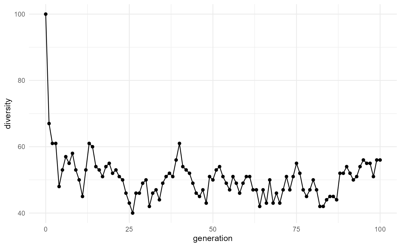
A plot can help users see whether the system becomes more diverse, less diverse, or more stable over time.
Diversity versus mutation
Mutation tends to introduce new variants. This can increase molecular diversity, especially when selection is weak or moderate.
sim_low_mutation <- simulate_abiogenesis(
  n_molecules = 100,
  generations = 100,
  mutation_rate = 0.001,
  selection_strength = 1,
  seed = 123
)

sim_high_mutation <- simulate_abiogenesis(
  n_molecules = 100,
  generations = 100,
  mutation_rate = 0.10,
  selection_strength = 1,
  seed = 123
)

head(sim_low_mutation)
## # A tibble: 6 × 6
## generation n_molecules mean_length mean_fitness diversity max_fitness
## <int> <int> <dbl> <dbl> <int> <dbl>
## 1 0 100 12.6 1.00 100 1.25
## 2 1 100 12.7 1.04 58 1.25
## 3 2 100 12.2 1.07 46 1.25
## 4 3 100 12.2 1.09 37 1.25
## 5 4 100 12.2 1.11 30 1.25
## 6 5 100 12.3 1.13 29 1.25
head(sim_high_mutation)## # A tibble: 6 × 6
## generation n_molecules mean_length mean_fitness diversity max_fitness
## <int> <int> <dbl> <dbl> <int> <dbl>
## 1 0 100 12.6 1.00 100 1.25
## 2 1 100 12.7 1.04 90 1.25
## 3 2 100 13.0 1.07 90 1.25
## 4 3 100 13.0 1.10 88 1.25
## 5 4 100 12.6 1.10 94 1.25
## 6 5 100 12.6 1.12 88 1.25Low mutation may preserve successful sequences but explore new possibilities slowly. High mutation may create many new variants, but it may also disrupt stable or successful molecules.
This creates a useful conceptual trade-off:
A system needs variation to evolve, but too much variation may prevent information from being preserved.
Diversity versus selection
Selection can reduce diversity if a small number of high-fitness molecules dominate. Mutation can increase diversity by generating new variants. The balance between mutation and selection is therefore central to molecular evolution.
weak_selection <- simulate_abiogenesis(
  n_molecules = 100,
  generations = 100,
  mutation_rate = 0.02,
  selection_strength = 0.2,
  seed = 123
)

strong_selection <- simulate_abiogenesis(
  n_molecules = 100,
  generations = 100,
  mutation_rate = 0.02,
  selection_strength = 3,
  seed = 123
)

head(weak_selection)
## # A tibble: 6 × 6
## generation n_molecules mean_length mean_fitness diversity max_fitness
## <int> <int> <dbl> <dbl> <int> <dbl>
## 1 0 100 12.6 1.00 100 1.25
## 2 1 100 13.2 1.01 74 1.25
## 3 2 100 13.1 0.993 67 1.25
## 4 3 100 13.0 1.01 64 1.25
## 5 4 100 12.3 1.02 56 1.25
## 6 5 100 12.6 1.05 52 1.25
head(strong_selection)## # A tibble: 6 × 6
## generation n_molecules mean_length mean_fitness diversity max_fitness
## <int> <int> <dbl> <dbl> <int> <dbl>
## 1 0 100 12.6 1.00 100 1.25
## 2 1 100 11.8 1.10 66 1.25
## 3 2 100 11.4 1.15 55 1.25
## 4 3 100 11.6 1.17 55 1.25
## 5 4 100 11.7 1.20 47 1.25
## 6 5 100 11.7 1.21 45 1.25In a weak-selection scenario, many molecular types may persist. In a strong-selection scenario, high-fitness molecules may dominate more quickly. This can reduce diversity, even while increasing average fitness.
Complexity and interpretation
It is tempting to say that higher diversity means higher complexity, but this is not always true. Complexity can involve diversity, organization, interaction, information storage, persistence, and functional integration.
For example:
- A random soup of molecules may have high diversity but little organization.
- A selected population may have lower diversity but stronger functional structure.
- An autocatalytic network may have moderate diversity but high interaction complexity.
- A protocell system may combine molecular diversity with compartment-level organization.
Therefore, diversity metrics should be used alongside other outputs such as:
- fitness,
- abundance,
- network structure,
- protocell dynamics,
- persistence over time,
- response to mutation and selection.
Teaching use
This tutorial can support discussions in:
- origin-of-life studies,
- evolutionary biology,
- systems biology,
- information theory,
- ecology and diversity metrics,
- complexity science.
Students can be asked to compare how different parameter choices affect diversity. This helps connect abstract concepts such as entropy and selection to visible simulation outputs.
Educational questions
Try changing mutation_rate and
selection_strength and ask:
- Which settings increase diversity?
- Which settings reduce diversity?
- Does stronger selection always reduce diversity?
- Does higher mutation always increase diversity?
- Can a system become more organized while becoming less diverse?
- Can a system become more diverse while becoming less organized?
Suggested exercises
- Create small and large molecular pools and compare their entropy.
- Run simulations with low and high mutation rates.
- Run simulations with weak and strong selection.
- Identify conditions that increase molecular diversity.
- Identify conditions that reduce molecular diversity.
- Discuss why diversity alone is not sufficient to define life.
- Compare diversity metrics with fitness trends.
- Compare molecular diversity with protocell and autocatalytic network behaviour.
- Propose an additional complexity metric that could be added to the package.
- Discuss how entropy in this model differs from thermodynamic entropy.
Important limitation
The metrics in this package are simplified educational tools. They do not fully capture biochemical complexity, functional organization, thermodynamics, or information storage in real prebiotic systems. They are best used as conceptual aids for exploring how diversity, mutation, and selection interact.