Getting Started with lifesimulatoR
Overview
lifesimulatoR provides simple simulation tools for
exploring how life-like behaviour might emerge from non-living chemical
systems.
The package does not attempt to reproduce real prebiotic chemistry in full detail. Instead, it uses symbolic molecules and toy models to make key origin-of-life ideas easier to teach, visualize, and explore.
The package can be used to ask conceptual questions such as:
- What happens when molecules replicate with errors?
- How can mutation and selection change a population?
- How can molecular diversity be measured?
- How might protocell-like compartments grow and divide?
- How can autocatalytic networks create self-reinforcing dynamics?
Basic workflow
A typical workflow begins with an initial pool of symbolic molecules. These molecules can then be mutated, replicated, selected, summarized, and plotted.
pool <- create_prebiotic_pool(
  n_molecules = 100,
  alphabet = c("A", "U", "G", "C"),
  min_length = 5,
  max_length = 20,
  seed = 123
)

head(pool)
## [1] "GGUGUUUGACUUAUGCAGG" "CAAAGCUGUAUGC" "AGGACGCUAGAAUGGCAG"
## [4] "GCUAUAACC" "AUAAGAUAGAGUCGCCUUG" "UUGGCAUUAUCA"The exact structure of the output depends on the current implementation of the package, but the goal is to represent a population of simple molecular sequences.
Run a complete molecular evolution simulation
The easiest entry point is simulate_abiogenesis().
result <- simulate_abiogenesis(
  n_molecules = 50,
  generations = 30,
  mutation_rate = 0.02,
  selection_strength = 1,
  seed = 1
)

head(result)
## # A tibble: 6 × 6
## generation n_molecules mean_length mean_fitness diversity max_fitness
## <int> <int> <dbl> <dbl> <int> <dbl>
## 1 0 50 13.4 1.06 50 1.25
## 2 1 50 12.9 1.12 40 1.25
## 3 2 50 12.5 1.15 34 1.25
## 4 3 50 12.5 1.19 28 1.25
## 5 4 50 12.3 1.18 33 1.25
## 6 5 50 12.4 1.19 34 1.25This simulation represents a simplified evolutionary process. Molecules vary, mutate, replicate, and undergo selection over repeated generations.
Plot simulation results
plot_simulation(result, x = "generation", y = "mean_fitness")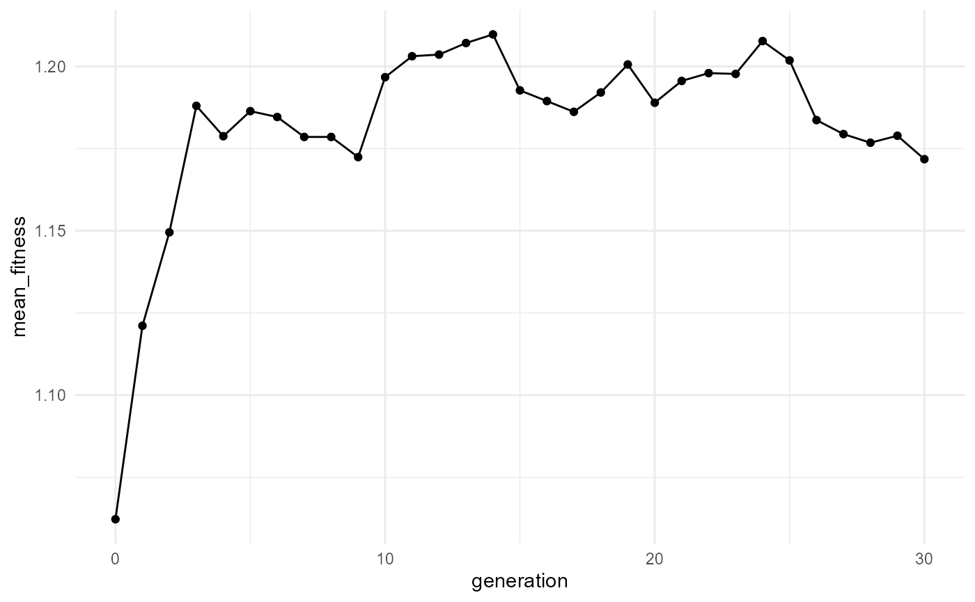
The plot is intended to help users see patterns over time, such as changes in fitness, diversity, abundance, or other simulation outputs.
If you are unsure which columns are available, inspect the result first:
names(result)## [1] "generation" "n_molecules" "mean_length" "mean_fitness" "diversity"
## [6] "max_fitness"Then choose suitable variables for plotting.
Explore molecular diversity
Molecular diversity is important because diverse systems can explore more possible structures and interactions.
summary_stats <- summarize_molecules(pool)

summary_stats
## # A tibble: 1 × 6
## generation n_molecules mean_length mean_fitness diversity max_fitness
## <dbl> <int> <dbl> <dbl> <int> <dbl>
## 1 0 100 12.6 1.00 100 1.25
pool_counts <- table(pool)

shannon_entropy(as.numeric(pool_counts))
## [1] 6.643856These functions help summarize a molecular population and estimate its diversity.
Autocatalytic networks
Autocatalytic networks are systems where molecules help produce other molecules in the same system. They are useful for exploring how chemical networks may become self-reinforcing.
net <- autocatalytic_network(
  n_types = 6,
  steps = 20,
  catalysis_probability = 0.2,
  seed = 2
)

head(net$time_series)
## # A tibble: 6 × 3
## step molecule abundance
## <int> <chr> <dbl>
## 1 0 M1 0.860
## 2 0 M2 0.356
## 3 0 M3 0.701
## 4 0 M4 0.235
## 5 0 M5 0.984
## 6 0 M6 0.367The returned object includes a time series of molecular abundances and a catalysis matrix.
net$catalysis_matrix## [,1] [,2] [,3] [,4] [,5] [,6]
## [1,] FALSE TRUE FALSE FALSE FALSE TRUE
## [2,] FALSE FALSE TRUE TRUE FALSE TRUE
## [3,] FALSE FALSE FALSE FALSE TRUE FALSE
## [4,] TRUE FALSE FALSE FALSE FALSE FALSE
## [5,] FALSE FALSE FALSE FALSE FALSE FALSE
## [6,] FALSE FALSE FALSE TRUE TRUE FALSEProtocell dynamics
Protocells are simplified cell-like compartments. They are useful for exploring how compartmentalization, growth, leakage, and division may matter in origin-of-life scenarios.
cells <- protocell_simulation(
  n_cells = 10,
  steps = 30,
  growth_rate = 0.2,
  division_threshold = 10,
  leakage_rate = 0.03,
  seed = 3
)

head(cells)
## # A tibble: 6 × 4
## step n_cells mean_abundance max_abundance
## <int> <int> <dbl> <dbl>
## 1 0 10 1.90 2.62
## 2 1 10 2.04 2.74
## 3 2 10 2.15 2.79
## 4 3 10 2.32 3.01
## 5 4 10 2.49 3.25
## 6 5 10 2.58 3.33You can plot protocell population size over time:
plot_simulation(cells, x = "step", y = "n_cells")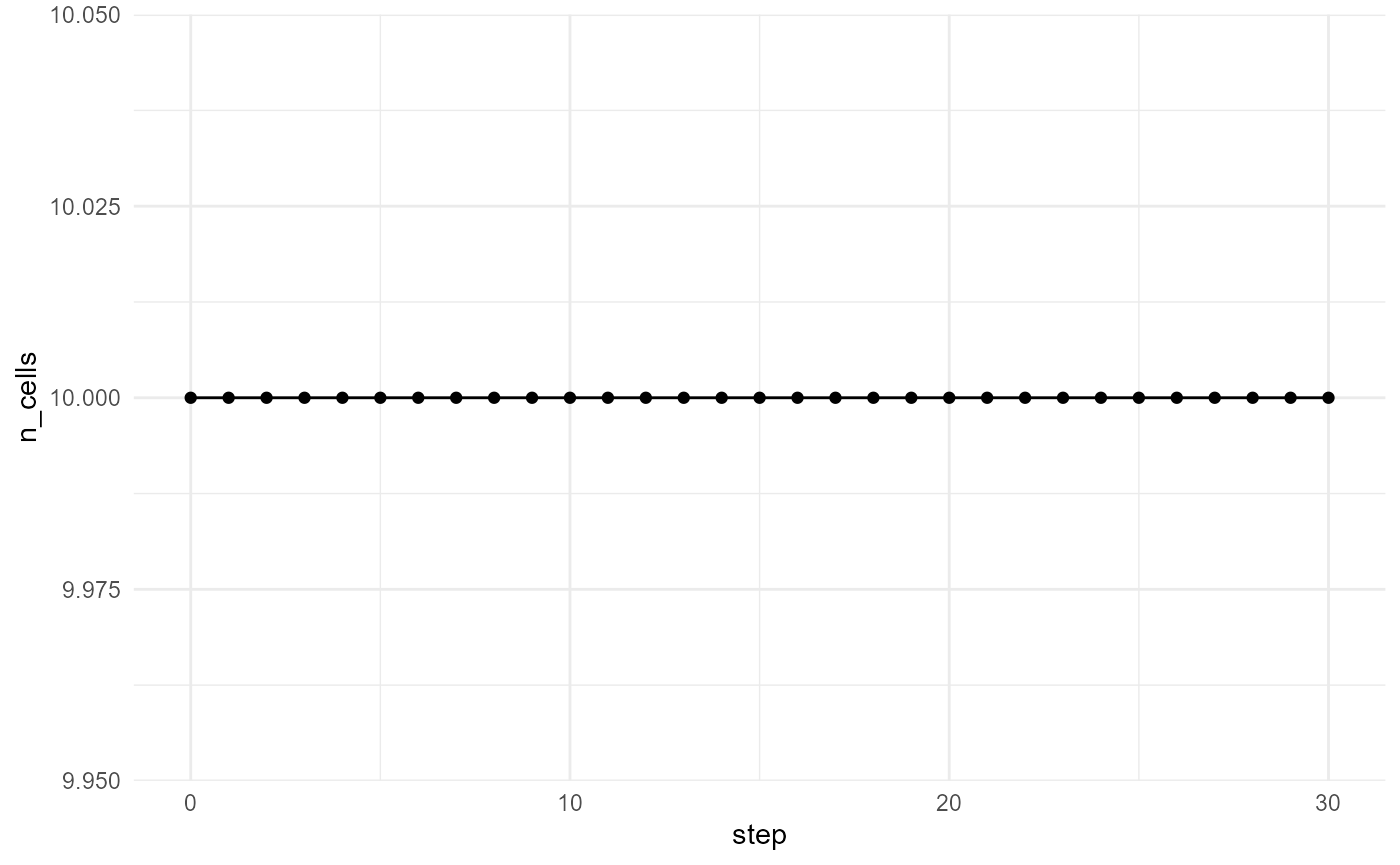
What to read next
After this introduction, the following tutorials provide more detail:
molecular-evolution.Rmddiversity-metrics.Rmdprotocells.Rmdautocatalytic-networks.Rmd
These concept tutorials explain the scientific ideas and show how the functions can be used together.
Important interpretation note
The simulations in lifesimulatoR are educational. A
result showing increasing fitness, diversity, or complexity should not
be interpreted as proof of a specific origin-of-life pathway.
Instead, the simulations are best used as conceptual demonstrations of mechanisms often discussed in origin-of-life research, including mutation, selection, replication, compartmentalization, autocatalysis, and emergence.