Molecular Evolution

Molecular Evolution with `lifesimulatoR`

Introduction

One of the central questions in origin-of-life research is how non-living chemical systems could begin to exhibit life-like behaviour. Modern life relies on molecules that store information, make copies of themselves, mutate, and undergo selection. DNA and RNA perform these roles today, but early life-like systems may have been much simpler.

In lifesimulatoR, molecular evolution is represented using symbolic sequences. A molecule may be represented by a sequence such as "AUGCUA". The letters A, U, G, and C are inspired by RNA chemistry, but the model is conceptual rather than chemically realistic.

The basic evolutionary workflow explored in this vignette is:

Create a prebiotic molecular pool.
Estimate molecular fitness.
Replicate molecules.
Introduce mutation.
Apply selection.
Repeat the process over many generations.
Observe how the population changes.

library(lifesimulatoR)

Create a prebiotic molecular pool

Every evolutionary system requires a starting population. Before mutation, replication, or selection can occur, there must first be a collection of molecules capable of varying from one another.

In origin-of-life research, this starting collection is often called a prebiotic pool.

A prebiotic pool represents an early chemical environment containing many different molecules. In reality these molecules could include amino acids, nucleotides, peptides, lipids, and other organic compounds. In lifesimulatoR, they are represented as symbolic sequences.

pool <- create_prebiotic_pool(
  n_molecules = 20,
  alphabet = c("A", "U", "G", "C"),
  min_length = 5,
  max_length = 12,
  seed = 123
)

head(pool)

## [1] "GGUGUUUGACU" "AUGCAGGACA"  "AGCUG"       "AUGCUA"      "GACGCUA"    
## [6] "AAUGGCAGAGC"

The output is a character vector where each element represents one symbolic molecule.

Why variation matters

Variation is essential because selection can only act when differences already exist.

If every molecule were identical, no molecule would have an advantage over any other.

Selection can only act on existing variation.

Understanding the parameters

n_molecules: number of molecules generated
alphabet: symbols used to construct molecules
min_length: minimum sequence length
max_length: maximum sequence length
seed: random seed for reproducibility

larger_pool <- create_prebiotic_pool(
  n_molecules = 100,
  alphabet = c("A", "U", "G", "C"),
  min_length = 5,
  max_length = 12,
  seed = 123
)

length(larger_pool)

## [1] 100

Exploring the pool

length(pool)

## [1] 20

nchar(pool)

##  [1] 11 10  5  6  7 11 10  5  5  8 12  8 12  7  7 11 10 10 12  6

data.frame(
  molecule = pool,
  length = nchar(pool)
)

##        molecule length
## 1   GGUGUUUGACU     11
## 2    AUGCAGGACA     10
## 3         AGCUG      5
## 4        AUGCUA      6
## 5       GACGCUA      7
## 6   AAUGGCAGAGC     11
## 7    AUAACCGAUA     10
## 8         GAUAG      5
## 9         GUCGC      5
## 10     UUGCUUGG      8
## 11 AUUAUCAAUGGA     12
## 12     UACUAGGC      8
## 13 UCGAUUCGUACG     12
## 14      GUUGAAC      7
## 15      UUUCUUU      7
## 16  CCUAUUUGCUG     11
## 17   GCAGGGAGGU     10
## 18   UGCGGUAUCC     10
## 19 AGGCCUCAGAGU     12
## 20       AGUCAG      6

Why the starting pool matters

The starting pool defines the raw material available to evolution.

A larger and more diverse pool may contain more possible variants for selection to act upon. A smaller or less diverse pool may limit exploration of molecular possibilities.

Calculate molecular fitness

Fitness is a simplified score representing how likely a molecule is to persist, replicate, or be selected.

In real chemistry, this would depend on factors such as:

stability
catalytic activity
environmental conditions
energy availability

example_sequence <- "AUGCUA"

molecule_fitness(example_sequence)

## [1] 0.8876282

Comparing fitness values

molecules <- c(
  "AUGC",
  "AAAAUUUU",
  "GCGCGC",
  "AUAUAUAUAUAU"
)

fitness <- molecule_fitness(molecules)

data.frame(
  molecule = molecules,
  fitness = fitness
)

##       molecule   fitness
## 1         AUGC 0.6993290
## 2     AAAAUUUU 1.0687308
## 3       GCGCGC 0.8876282
## 4 AUAUAUAUAUAU 1.2500000

Questions to consider:

Should longer molecules have higher fitness?
Should catalytic motifs increase fitness?
How should fitness be represented in origin-of-life simulations?

Mutation: changing molecular sequences

Mutation introduces novelty into a molecular population.

Without mutation, populations may replicate, but they cannot easily explore new sequence space.

In origin-of-life models, mutation can represent:

copying errors
chemical modifications
structural rearrangements

Mutation can be explored at two levels:

Individual sequences
Entire populations

Mutate one sequence

set.seed(2)

original <- "AUGCAUGCAUGC"

mutated <- mutate_sequence(
  sequence = original,
  alphabet = c("A", "U", "G", "C"),
  mutation_rate = 0.2
)

data.frame(
  original = original,
  mutated = mutated
)

##       original      mutated
## 1 AUGCAUGCAUGC UUGGAUACAUGC

A mutation rate of 0.2 means each position has a relatively high chance of being altered.

Low versus high mutation rate

set.seed(3)

low_mutation <- mutate_sequence(
  sequence = "AUGCAUGCAUGC",
  alphabet = c("A", "U", "G", "C"),
  mutation_rate = 0.01
)

set.seed(3)

high_mutation <- mutate_sequence(
  sequence = "AUGCAUGCAUGC",
  alphabet = c("A", "U", "G", "C"),
  mutation_rate = 0.40
)

data.frame(
  mutation_rate = c(0.01, 0.40),
  mutated_sequence = c(low_mutation, high_mutation)
)

##   mutation_rate mutated_sequence
## 1          0.01     AUGCAUGCAUGC
## 2          0.40     GUCCAUCCAUGC

A low mutation rate usually preserves the original sequence.

A high mutation rate introduces more variation, but excessive mutation may disrupt useful molecular patterns.

Variation is necessary for evolution, but too much variation can prevent useful information from being preserved.

Mutate a population

set.seed(4)

molecules <- c("AUGC", "UUUU", "GCGC", "AAAA")

mutated_population <- mutate_population(
  molecules = molecules,
  mutation_rate = 0.2
)

data.frame(
  before = molecules,
  after = mutated_population
)

##   before after
## 1   AUGC  AGGC
## 2   UUUU  UUUU
## 3   GCGC  UCGU
## 4   AAAA  AAAA

Some molecules remain unchanged, while others accumulate mutations.

Replication and selection

Replication allows successful molecules to become more common.

Selection means that molecules with higher fitness have a greater chance of contributing to future generations.

molecules <- c(
  "AUGC",
  "AAAAUUUU",
  "GCGCGC",
  "AUAUAUAUAUAU"
)

next_generation <- replicate_molecules(
  molecules = molecules,
  n_molecules = 20,
  selection_strength = 1
)

next_generation

##  [1] "GCGCGC"       "GCGCGC"       "AUGC"         "AAAAUUUU"     "AAAAUUUU"    
##  [6] "GCGCGC"       "AUGC"         "AAAAUUUU"     "AUGC"         "AAAAUUUU"    
## [11] "AAAAUUUU"     "AAAAUUUU"     "AUAUAUAUAUAU" "AUGC"         "GCGCGC"      
## [16] "AAAAUUUU"     "AUGC"         "AAAAUUUU"     "GCGCGC"       "AAAAUUUU"

Selection strength

The parameter selection_strength controls how strongly fitness influences replication.

0 = neutral drift
low values = weak selection
high values = strong selection

Compare neutral drift and selection

set.seed(1)

neutral <- replicate_molecules(
  molecules = molecules,
  n_molecules = 100,
  selection_strength = 0
)

set.seed(1)

selected <- replicate_molecules(
  molecules = molecules,
  n_molecules = 100,
  selection_strength = 2
)

table(neutral)

## neutral
##     AAAAUUUU AUAUAUAUAUAU         AUGC       GCGCGC 
##           20           21           27           32

table(selected)

## selected
##     AAAAUUUU AUAUAUAUAUAU         AUGC       GCGCGC 
##           29           37           11           23

As selection strength increases, fitter molecules become more common.

Evolve one generation

The function evolve_generation() combines:

fitness
replication
mutation
selection

into a single evolutionary step.

next_generation <- evolve_generation(
  molecules = pool,
  mutation_rate = 0.02,
  selection_strength = 1
)

head(next_generation)

## [1] "GGUGUUUGACU" "AUAACCGAUA"  "AAUGGCAGAGC" "AGUCAG"      "UUGCUUGG"   
## [6] "CCUAUUUGCUG"

One generation illustrates the mechanism. Many generations reveal longer-term trends.

Simulate abiogenesis-like molecular evolution

The main simulation function is simulate_abiogenesis().

It starts with a random molecular pool and repeatedly applies:

replication
mutation
selection

over many generations.

sim <- simulate_abiogenesis(
  n_molecules = 100,
  generations = 200,
  mutation_rate = 0.01,
  selection_strength = 1,
  seed = 10
)

head(sim)

## # A tibble: 6 × 6
##   generation n_molecules mean_length mean_fitness diversity max_fitness
##        <int>       <int>       <dbl>        <dbl>     <int>       <dbl>
## 1          0         100        12.6         1.02       100        1.25
## 2          1         100        12.4         1.08        69        1.25
## 3          2         100        12.7         1.08        58        1.25
## 4          3         100        12.7         1.11        55        1.25
## 5          4         100        13.0         1.12        53        1.25
## 6          5         100        13.0         1.13        47        1.25

tail(sim)

## # A tibble: 6 × 6
##   generation n_molecules mean_length mean_fitness diversity max_fitness
##        <int>       <int>       <dbl>        <dbl>     <int>       <dbl>
## 1        195         100          12         1.25        35        1.25
## 2        196         100          12         1.25        37        1.25
## 3        197         100          12         1.25        37        1.25
## 4        198         100          12         1.25        39        1.25
## 5        199         100          12         1.25        42        1.25
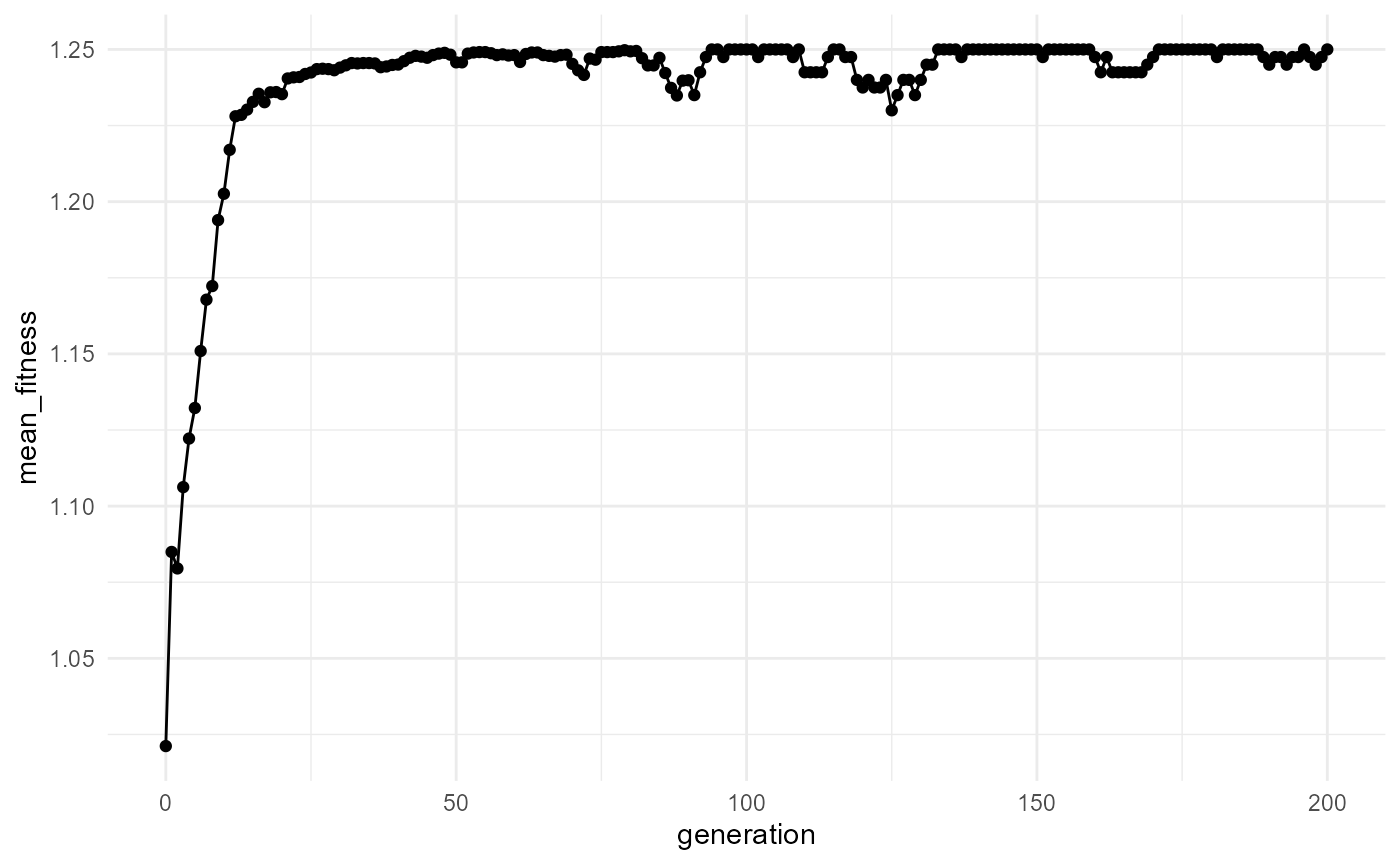
## 6        200         100          12         1.25        39        1.25

The output is a tibble summarizing population-level changes through time.

Visualize results

Plot mean fitness

plot_simulation(
  sim,
  x = "generation",
  y = "mean_fitness"
)

Plot diversity

plot_simulation(
  sim,
  x = "generation",
  y = "diversity"
)

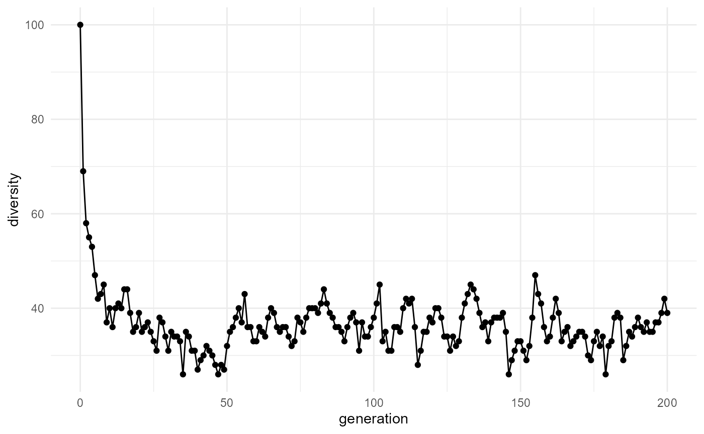
Plots can help answer questions such as:

Does mean fitness increase?
Does diversity increase or decrease?
Does the population stabilize?
Does selection lead to dominance by certain molecule types?

Parameter experiments

Experiment 1: mutation rate

low_mutation <- simulate_abiogenesis(
  n_molecules = 100,
  generations = 100,
  mutation_rate = 0.005,
  selection_strength = 1,
  seed = 123
)

high_mutation <- simulate_abiogenesis(
  n_molecules = 100,
  generations = 100,
  mutation_rate = 0.10,
  selection_strength = 1,
  seed = 123
)

Compare the results.

Questions:

Which simulation produces more diversity?
Which preserves information more effectively?

Experiment 2: selection strength

weak_selection <- simulate_abiogenesis(
  n_molecules = 100,
  generations = 100,
  mutation_rate = 0.02,
  selection_strength = 0.2,
  seed = 123
)

strong_selection <- simulate_abiogenesis(
  n_molecules = 100,
  generations = 100,
  mutation_rate = 0.02,
  selection_strength = 3,
  seed = 123
)

Questions:

Does stronger selection increase fitness?
Does stronger selection reduce diversity?

Interpretation

This tutorial demonstrates a simplified model of molecular evolution.

Key concepts include:

Variation
Fitness
Replication
Mutation
Selection
Population-level change

The model is intentionally simple. It does not simulate:

real chemistry
RNA folding
thermodynamics
energy flow
detailed reaction kinetics

Instead, it provides an educational framework for exploring how life-like evolutionary dynamics may emerge.

Suggested exercises

Run simulations with mutation rates of 0, 0.01, 0.05, and 0.20.
Compare weak and strong selection.
Change the alphabet used to generate molecules.
Compare short and long molecule populations.
Modify the fitness function.
Compare neutral drift and selection.
Discuss what would be needed to make the model chemically realistic.
Compare molecular evolution with protocell models.
Compare molecular evolution with autocatalytic network models.
Debate whether replication-first, metabolism-first, or compartment-first models provide the best explanation for the origin of life.