Agents and Traits Tutorial
Source:vignettes/agents-and-traits-tutorial.Rmd
agents-and-traits-tutorial.RmdPurpose
This tutorial introduces create_agents().
Artificial-life simulations often begin with a population of agents.
Agents are simplified individuals with states, traits, and sometimes
locations.
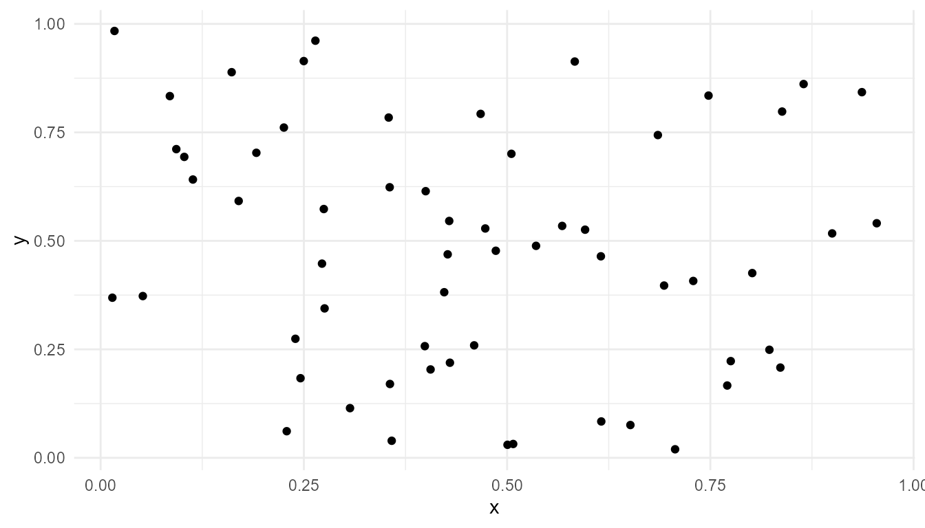
In this tutorial, you will learn how to create agents, inspect their traits, visualize their positions, and summarize trait variation.
Create a population
agents <- create_agents(
  n_agents = 60,
  seed = 10
)

head(agents)
#>   agent          x          y    energy      speed efficiency
#> 1     1 0.50747820 0.03188816 0.8143608 0.04037269  0.5425513
#> 2     2 0.30676851 0.11446759 0.9315736 0.05405764  0.5643500
#> 3     3 0.42690767 0.46893548 0.8754516 0.04936521  0.3639694
#> 4     4 0.69310208 0.39698674 1.0510173 0.02608839  0.4801494
#> 5     5 0.08513597 0.83361919 1.1599565 0.06247362  0.5619303
#> 6     6 0.22543662 0.76112174 1.1824189 0.03170391  0.7068210
#>   reproduction_threshold age alive
#> 1               1.660511   0  TRUE
#> 2               1.574442   0  TRUE
#> 3               1.586208   0  TRUE
#> 4               1.539516   0  TRUE
#> 5               1.550912   0  TRUE
#> 6               1.487745   0  TRUE
Inspect the output
str(agents)
#> 'data.frame':    60 obs. of  9 variables:
#>  $ agent                 : int  1 2 3 4 5 6 7 8 9 10 ...
#>  $ x                     : num  0.5075 0.3068 0.4269 0.6931 0.0851 ...
#>  $ y                     : num  0.0319 0.1145 0.4689 0.397 0.8336 ...
#>  $ energy                : num  0.814 0.932 0.875 1.051 1.16 ...
#>  $ speed                 : num  0.0404 0.0541 0.0494 0.0261 0.0625 ...
#>  $ efficiency            : num  0.543 0.564 0.364 0.48 0.562 ...
#>  $ reproduction_threshold: num  1.66 1.57 1.59 1.54 1.55 ...
#>  $ age                   : num  0 0 0 0 0 0 0 0 0 0 ...
#>  $ alive                 : logi  TRUE TRUE TRUE TRUE TRUE TRUE ...
The main columns include:
| Column | Meaning |
|---|---|
agent |
Agent identifier |
x, y
|
Position in the world |
energy |
Available energy |
speed |
Movement capacity |
efficiency |
Ability to convert resources into energy |
reproduction_threshold |
Energy needed for reproduction |
age |
Agent age |
alive |
Survival status |
Summarize traits
summary(agents[, c("energy", "speed", "efficiency", "reproduction_threshold")])
#>      energy           speed           efficiency     reproduction_threshold
#>  Min.   :0.7513   Min.   :0.01000   Min.   :0.2795   Min.   :1.256
#>  1st Qu.:0.9002   1st Qu.:0.03243   1st Qu.:0.3915   1st Qu.:1.453
#>  Median :1.0374   Median :0.04718   Median :0.4804   Median :1.511
#>  Mean   :1.0114   Mean   :0.04711   Mean   :0.4853   Mean   :1.511
#>  3rd Qu.:1.1169   3rd Qu.:0.06252   3rd Qu.:0.5575   3rd Qu.:1.582
#>  Max.   :1.3331   Max.   :0.07942   Max.   :0.7068   Max.   :1.743
Measure trait diversity
measure_life_like_complexity(
  agents,
  trait_col = "efficiency"
)
#>    n unique_values entropy     mean         sd temporal_variability
#> 1 60            60 2.97102 0.485314 0.09663056                   NA
#>   mean_abs_change
#> 1              NA
Compare populations
Create two populations with different trait variability.
low_variation <- create_agents(
  n_agents = 60,
  trait_sd = 0.03,
  seed = 10
)

high_variation <- create_agents(
  n_agents = 60,
  trait_sd = 0.20,
  seed = 10
)

rbind(
  low_variation = measure_life_like_complexity(low_variation, trait_col = "efficiency"),
  high_variation = measure_life_like_complexity(high_variation, trait_col = "efficiency")
)
#>                 n unique_values entropy      mean         sd
#> low_variation  60            60 2.97102 0.4955942 0.02898917
#> high_variation 60            60 2.97102 0.4706281 0.19326112
#>                temporal_variability mean_abs_change
#> low_variation                    NA              NA
#> high_variation                   NA              NA
Interpretation
Higher trait variability gives the population more initial diversity. In artificial-life models, variation matters because selection and adaptation require differences among individuals.
However, variation alone is not evolution. Evolution-like dynamics also require inheritance, differential persistence, and change across generations.
Suggested exercises
- Increase
n_agentsand inspect how the output changes. - Change
energy_meanand observe the distribution of energy. - Change
trait_sdand compare efficiency summaries. - Ask which traits might matter under resource competition.
Key takeaway
create_agents() provides the starting population for
artificial-life simulations. The agents are simplified units, but they
make it possible to explore trait variation, energy, and
individual-level differences.