Cellular Automata and Local Rules
Source:vignettes/cellular-automata-theory.Rmd
cellular-automata-theory.RmdPurpose
This article explains why cellular automata are central examples in the study of emergence. A cellular automaton is a simple computational system made of cells whose states are updated according to local rules. Despite their simplicity, cellular automata can generate highly structured, unpredictable, and computation-like patterns (Wolfram 2002; Langton 1990).
The purpose of this chapter is to show how
simulate_cellular_automata() can be used to explore the
relationship between local rules and global patterns.
The guiding question is:
How can a simple local update rule generate complex system-level behavior?
What is a cellular automaton?
A cellular automaton consists of a set of cells arranged in space. Each cell has a state, and the state of each cell changes over time according to a rule.
In an elementary cellular automaton, the structure is especially simple:
- cells are arranged in one dimension;
- each cell has a binary state, usually
0or1; - each cell updates based on itself and its immediate neighbors;
- the same rule is applied to every cell at every time step.
Although this setup is simple, the resulting patterns can be surprisingly rich.
Local rules and global patterns
Cellular automata are useful because they make the logic of emergence visible. Each cell follows a local rule. It does not know the full system. It does not plan the future pattern. It responds only to its immediate neighborhood.
Yet when the rule is applied repeatedly across many cells, a global pattern appears.
This is the core emergent lesson:
No individual cell contains the global pattern, but the pattern arises from the repeated local interactions of many cells.
In this sense, cellular automata provide a clear example of how system-level structure can arise without central control.
Elementary cellular automata
In elementary cellular automata, each cell’s next state is determined by three values:
- the left neighbor,
- the cell itself,
- the right neighbor.
Because each of these values can be either 0 or
1, there are eight possible neighborhood
configurations:
111 110 101 100 011 010 001 000A rule specifies what the next state should be for each of these
eight configurations. Since each output can also be 0 or
1, there are 256 possible elementary cellular automaton
rules.
Rules are usually identified by number, such as Rule 30, Rule 90, or Rule 110.
Relation to the package
The function simulate_cellular_automata() implements
elementary cellular automata in a simplified educational form.
| Theoretical concept | Package representation |
|---|---|
| Cell | Position in a one-dimensional grid |
| Cell state | Binary value, usually 0 or 1
|
| Local neighborhood | Cell plus nearby cells |
| Update rule |
rule argument |
| Time evolution | steps |
| Global pattern | Raster visualization over time |
The function helps learners see how changing the local rule changes the global pattern.
Simulation example: Rule 30
Rule 30 is often used as an example of how a simple deterministic rule can produce complex, irregular-looking behavior.
rule30 <- simulate_cellular_automata(
  rule = 30,
  n_cells = 81,
  steps = 80
)

plot_emergence_sim(
  rule30,
  x = "cell",
  y = "step",
  value = "state",
  type = "raster"
)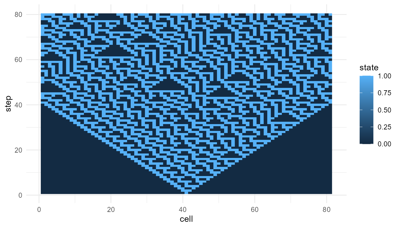
Interpretation of Rule 30
The pattern produced by Rule 30 is generated entirely by the local update rule. No randomness is added during the update process, yet the resulting pattern can appear irregular and difficult to predict visually.
This makes Rule 30 useful for teaching an important point:
Deterministic systems can produce complex patterns.
The complexity is not imposed from outside. It arises through repeated local updating.
Rule 110 and computation
Rule 110 is especially important because it has been associated with complex structures and computation-like behavior in cellular automata research (Wolfram 2002; Langton 1990).
rule110 <- simulate_cellular_automata(
  rule = 110,
  n_cells = 81,
  steps = 80
)

plot_emergence_sim(
  rule110,
  x = "cell",
  y = "step",
  value = "state",
  type = "raster"
)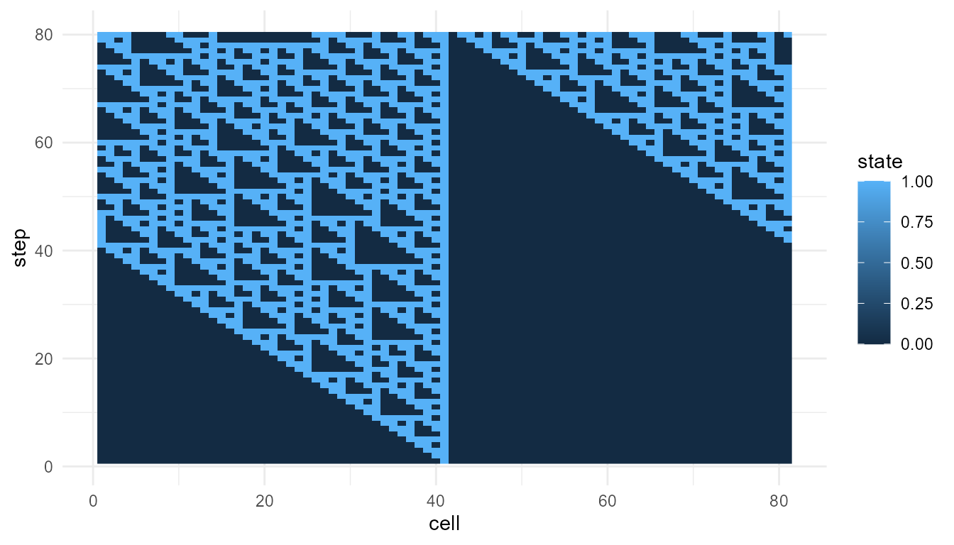
Interpretation of Rule 110
Rule 110 often produces localized structures that move, interact, or persist over time. These structures are important because they suggest that simple rule-based systems can support rich dynamics.
This does not mean that Rule 110 is alive or conscious. Rather, it shows that simple computational systems can generate patterns with enough structure to support computation-like interpretation.
For emergence studies, Rule 110 is useful because it occupies a middle ground between simple order and complete disorder.
Order, randomness, and complexity
Cellular automata are useful because different rules can produce different kinds of behavior.
Some rules produce uniform or repetitive patterns. Others produce random-looking patterns. Others produce structured complexity.
This helps illustrate an important idea in complexity science:
Emergence often appears between rigid order and complete randomness.
If a system is too ordered, little novelty appears. If it is too random, stable structure may not persist. Interesting emergent behavior often appears in systems that combine stability and change.
Comparing rules
The following example compares different rules.
rule90 <- simulate_cellular_automata(
  rule = 90,
  n_cells = 81,
  steps = 80
)

rule150 <- simulate_cellular_automata(
  rule = 150,
  n_cells = 81,
  steps = 80
)

head(rule90)
#>   step cell state
#> 1    1    1     0
#> 2    1    2     0
#> 3    1    3     0
#> 4    1    4     0
#> 5    1    5     0
#> 6    1    6     0
head(rule150)
#>   step cell state
#> 1    1    1     0
#> 2    1    2     0
#> 3    1    3     0
#> 4    1    4     0
#> 5    1    5     0
#> 6    1    6     0
Rule 90 is often associated with nested, triangular structure. Rule 150 can also generate structured patterns, depending on initial conditions.
The important point is that small changes in rule structure can produce large changes in system-level behavior.
Measuring cellular automata patterns
Visual inspection is important, but simple metrics can help compare outputs.
measure_emergence(
  rule30,
  value_col = "state",
  time_col = "step"
)
#>      n unique_states shannon_entropy mean_value  sd_value temporal_variability
#> 1 6480             2       0.9612044  0.3845679 0.4865305            0.1640558
#>   mean_absolute_change
#> 1           0.07110486
Metrics such as diversity, entropy, or temporal change can help learners compare patterns across rules.
However, these metrics should be interpreted carefully. They do not fully define emergence. They provide summaries that support comparison.
Sensitivity to initial conditions
Cellular automata can also show how initial conditions matter. The same rule may produce different patterns depending on the starting configuration.
In many emergent systems, both the rule and the initial state matter. A system’s future is shaped by its dynamics and its history.
rule30_a <- simulate_cellular_automata(
  rule = 30,
  n_cells = 81,
  steps = 80
)

rule30_b <- simulate_cellular_automata(
  rule = 30,
  n_cells = 81,
  steps = 80
)

head(rule30_a)
#>   step cell state
#> 1    1    1     0
#> 2    1    2     0
#> 3    1    3     0
#> 4    1    4     0
#> 5    1    5     0
#> 6    1    6     0
head(rule30_b)
#>   step cell state
#> 1    1    1     0
#> 2    1    2     0
#> 3    1    3     0
#> 4    1    4     0
#> 5    1    5     0
#> 6    1    6     0
If your function uses a fixed default initial condition, the same rule will reproduce the same pattern. If random initial conditions are added in future versions, this section can be expanded to compare how starting states influence the outcome.
Cellular automata and emergence
Cellular automata illustrate several core features of emergence:
- local rules can generate global patterns;
- simple components can produce complex behavior;
- no central controller is required;
- repeated updating matters;
- visual patterns can be difficult to predict from the rule alone;
- small rule differences can produce major system differences.
These features make cellular automata powerful teaching tools.
Cellular automata and artificial life
Cellular automata have played an important role in artificial life and complexity science. They provide a way to explore how life-like organization, computation, and pattern formation might arise in simple rule-based systems.
They do not model real biological life in detail. However, they help clarify how organized behavior can arise from local interactions.
This makes them relevant to broader questions about:
- origin of life;
- self-organization;
- artificial life;
- computation;
- complex systems;
- emergence and consciousness.
Relation to other package functions
| Function | Relationship to cellular automata |
|---|---|
simulate_cellular_automata() |
Generates local-rule-based patterns |
simulate_self_organization() |
Models spatial pattern formation through feedback and diffusion |
simulate_agent_interactions() |
Models emergence from interacting agents |
simulate_network_growth() |
Models emergence of relational structure |
measure_emergence() |
Summarizes diversity, entropy, or change |
plot_emergence_sim() |
Visualizes cellular automata and other emergent outputs |
Cellular automata provide one of the clearest examples of emergence, while the other functions show different pathways to system-level organization.
What the model captures
The function captures several important ideas:
- cells update based on local neighborhoods;
- repeated local rules generate global patterns;
- deterministic systems can produce complex behavior;
- rule changes can produce different system-level structures;
- visual patterns can be used to teach emergence.
These features make cellular automata especially useful in introductory complexity education.
What the model does not capture
The model is intentionally simplified. It does not include:
- continuous space;
- continuous time;
- physical forces;
- metabolism;
- adaptation;
- learning;
- evolution;
- real biological cells;
- environmental feedback.
The cells in cellular automata are abstract computational units, not biological cells.
Responsible interpretation
It is better to say:
The simulation illustrates how local update rules can generate emergent patterns.
than:
The simulation explains all emergence.
It is better to say:
Cellular automata are useful toy models for studying local-rule dynamics.
than:
Cellular automata are realistic models of life or consciousness.
Careful interpretation matters because cellular automata are powerful but highly abstract.
Educational use
This chapter can support several classroom or self-study questions:
- How does a local rule generate a global pattern?
- Why do different rules produce different structures?
- Can deterministic systems produce complex outcomes?
- What is the difference between randomness and complexity?
- Why is Rule 110 important?
- What do cellular automata reveal about emergence?
- What do they leave out?
These questions help learners understand cellular automata as conceptual tools for thinking about emergence.
Key takeaway
Cellular automata show how simple local rules can produce complex global patterns. They are among the clearest and most teachable examples of emergence.
simulate_cellular_automata() provides a simplified way
to explore this idea in R. Its value lies not in realism, but in
clarity: it makes the relationship between local rule and global pattern
visible.